Under the US EPA's Stage 2 Disinfectant by-product Rule, utilities are required to identify locations in their water distribution systems that are likely to have high concentrations of disinfectant by-products such as Trihalomethanes and Haloacetic acids. Both of these are associated with high water age.

In general the easiest and most beneficial way to comply with the EPA regulations is to conduct a system specific study and the most expedient way of doing this is to construct a calibrated, detailed extended period simulation model which can identify locations in the system with high water age. The details of the requirements for such a model are provided in "System Specific Study Using a Distribution System Hydraulic Model" available at:

http://www.epa.gov/safewater/disinfection/stage2/compliance.html

HAMMER CONNECT can be used to comply with these regulations. Special tools have been added to assist in IDSE (Initial Distribution System Evaluation) studies. They are described below:

The utility must demonstrate that it has a well calibrated model.

From the regulations:

"A description of all calibration activities undertaken (or to be undertaken). This must include, if calibration is complete,

• A graph of predicted tank levels versus measured tank levels for the storage facility with the highest residence time in each pressure zone.
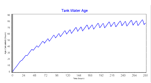
• A time series graph of water age results for the storage facility with the highest residence time in your system showing predictions for the entire EPS simulation period (i.e. from time zero until the time it takes for the model to reach a consistently repeating pattern of residence time)."

The graphing tools for displaying field observations alongside of model results have been improved for Select Upgrade 1 to make it easier to import field data using copy/paste commands from data sources such as spreadsheets and data base files

The utility's model used in an IDSE study must contain at least 50% of the pipe length in the real system and at least 75% of the pipes volume.

EPA regulations require:

• At least 50 percent of total pipe length in the distribution system.
• At least 75 percent of the pipe volume in the distribution system.
• All 12-inch diameter and larger pipes.
• All 8-inch diameter and larger pipes that connect pressure zones, mixing zones from different sources, storage facilities, major demand areas, pumps, and control valves, or are known or expected to be significant conveyors of water.
• All 6-inch diameter and larger pipes that connect remote areas of a distribution system to the main portion of the system or are known or expected to be significant conveyors of water.
• All storage facilities, with controls or settings applied to govern the open/closed status of the facility that reflect standard operations.
• All active pump stations, with realistic controls or settings applied to govern their on/off status that reflect standard operations.
• All active control valves or other system features that could significantly affect the flow of water through the distribution system (e.g., interconnections with other systems, pressure reducing valves between pressure zones).

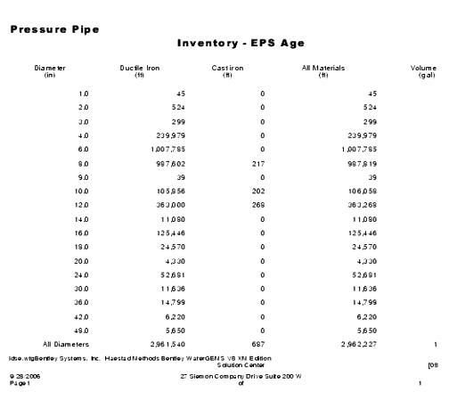
A table providing information on the total length of pipe and volume of water in the model is available by clicking the Report menu and selecting Pressure Pipe Inventory. This inventory can be printed using the Print Preview button at the top of the display or copied to the clipboard for use in other documents by highlighting all columns and hitting CTRL-C. If the columns are so wide that the wrapping of the columns does not look attractive, the user can resize the column widths by grabbing the edges of the column and sliding the border to a desired position.

Below is an example of one such table:

The utility must be able to calculate, display and perform statistics on water age.

This is done by setting up an EPS run for a long duration (e.g. one week). The user then selects "Age" as the calculation type in the calculation options. The duration of the run should be sufficiently long such that the water age is not continuing to increase in the system at the end of the run. Selecting a good initial water age for the tanks can reduce the length of time required to reach a recurring pattern.

The user also needs the ability to calculate some statistics after an water age EPS run to include average water age at each element between hours a and b.

Average water age over the final 24 hours of an EPS run can be calculated using the Post Calculation Processor which can be found under the Analysis menu.

An example is shown below. To determine the average water age at all junctions for the last 24 hour of, for instance, a 144 hour run, set the following values:

• Start time: 120
• Stop Time: 144
• Statistic Type: Mean (Time weighted)
• Results Property (field): Age (Calculated)
• Output Property (field): AveAge
• Operation: Set

Then use the browser above the bottom pane to select all the junctions for which average age is to be calculated. It's recommended to create a selection set with the elements desired before entering the Post Calculation Processor.

Mean (Time weighted) takes into account the fact that not all time steps are of the same size.

Result property (field) means that the Age (Calculated) property (attribute) in the model will be used to determine the average age.

Output property (field) means that the resulting average age for each selected element will be placed in a user defined property (field) called AveAve. . Instructions on establishing a user defined output property (field) can be found under User Data Extensions Dialog Box.

Once the average age property has been determined for each element, it is possible to color, annotate, contour or perform other HAMMER CONNECT operations on that property as with any other user defined property. The user can sort on this property (attribute) in FlexTables and determine the median. This helps the user comply with the portion of the regulation that states:

"Average residence time is the average age of water delivered to customers in a distribution system. Average residence time is not simply one-half the maximum residence time. Ideally, it should be a flow-weighted or population-weighted estimate. The model results for water age/DBP concentration can be used to determine the average residence time for your system. One option for doing this is to list the water age/DBP concentration results in ranked order for the entire system..."

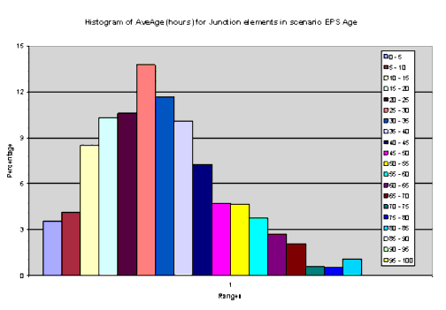
A histogram plot sorts the water age results into groups and shows the percentage of nodes with water ages falling within the given range.

A histogram can be created using a WaterObjects.NET feature which enables the user to utilize the graphing capability of Excel to create the histogram. The user starts Excel and if HAMMER CONNECT was loaded correctly, picks HAMMER CONNECT > Import Data and will then enter a browser titled "Please select a Water Model." The user browses to the file corresponding to the model under consideration. The screen below opens. (If model results have not been calculated for the base scenario for the model the user will be asked if a calculation is desired.)

The fields in this dialog are described below for the case of creating a IDSE histogram The fields in this dialog are described below for the case of creating a IDSE histogram:

• Source model: Full path name of model file
• Scenario: Name of Scenario to be imported
• Time step: Time step to be imported (value of average age is same for any time step)
• Element type: Average age is calculated at junctions
• Property (attribute): Average age for this case but any property (attribute) can be imported
• Use selection set: check if user only wants to import a subset of junctions
• Select set: name of selection set if previous box is checked
• Active elements only: Check if inactive elements are to be ignored which is usually the case

The next group of settings refers to the Histogram to be created:

• Create histogram: Check if histogram is desired
• Histogram Name: Name of worksheet in which histogram is placed
• Number of intervals: Number of bars in histogram
• Specify min/max?: If checked, user can override default values of ranges (recommended)
• Minimum: Minimum value of lowest interval
• Maximum: Maximum value of highest interval
  Note: The "Get min/max" button will populate the Minimum and Maximum boxes and act as defaults. (The Minimum and maximum fields enable the user to create histograms which have round number a breakpoints instead of the default ranges which can be on the order of 18.34-24.67.)
• Histogram type: The vertical axis can be labeled by number of points (Junction elements) in each interval or percentage of point in each interval.

The Import button begins the importing of values from the model file into the spreadsheet and creates the histogram if that box is checked. The final histogram will look like the one below for 10 intervals with Frequency selected.

Here is an example with a large number of intervals and percentage of points as the axis: